library(intsvy) # for complex survey analysis
library(dplyr) # for data manipulation
library(tidyr) # for data reshaping
library(knitr) # for creating pretty html tables
library(ggplot2) # for data visualization

# Set data path to your data directory
data_path <- "data/PISA/"PISA case study analysis with intsvy
Assessing the effects of gender and country on reading skills; the effects of country and the size of place of residence on science skills; and the effect of SES on the probability of missing school for over 3 months due to problematic behavior. Descriptive statistics, as well as linear and logistic regression analyses are utilized in the tutorial.
1 Introduction
This document demonstrates the preparation and analysis of the PISA 2022 (Programme for International Student Assessment 2022) dataset using the R intsvy package. PISA assesses the achievements of 15-year-old students in mathematics, reading, and science.
The analysis presented here focuses on differences in reading skills by gender and country.
We will also assess the impact of country and the size of the place of residence on science skills.
Lastly, we will evaluate the relationship between socioeconomic status (SES) and missing school for over 3 months due to problematic behavior, such as violence or drug use.
The analysis will be performed using the intsvy package, which is designed for analyzing complex survey data with replication weights.
Note
More about the intsvy package can be found in our tutorial.
2 Setup
First, let’s load the required packages and set up our environment:
3 Data download, loading and preparation
Data Download
The data can be downloaded from the PISA public data repository.
You should download data in .sav (SPSS file format) and save it in a chosen directory.
The select.merge() function from the intsvy package will accept only .sav files.
The variables we will focus on are:
ST004D01T- student’s genderCNT- country nameESCS- socioeconomic status scoreSC001Q01TA- size/type of the place of residenceST261Q02JA- miss school for 3+ months: I was suspended (e.g. for violence, use or sell drugs) [Yes/No]PV1READtoPV10READ- plausible values for reading scorePV1SCIEtoPV10SCIE- plausible values for science score
We will use the pisa.select.merge() function to read and merge student and school datasets. We will focus on four countries: Morocco, Finland, Singapore, and Poland.
pisa22 <- pisa.select.merge(
  folder = data_path,
  school.file = "CY08MSP_SCH_QQQ.SAV",
  student.file = "CY08MSP_STU_QQQ.SAV",
  student = c("ESCS", "ST004D01T", "ST261Q02JA"),
  school = c("SC001Q01TA"),
  countries = c("Finland", "Poland", "Singapore", "Morocco")
)
We have the dataset ready for analysis. Let’s proceed.
4 Differences in scores in reading by country and gender
In this part, we will compare the means and standard deviations of reading results by country and gender.
Mean and standard deviation of reading by country and gender
# Mean scores in reading by country and gender in PISA
descriptives <- pisa.mean.pv(
  pvlabel = paste0("PV", 1:10, "READ"),
  by = c("CNT", "ST004D01T"),
  data = pisa22
)

kable(descriptives,
  digits = 2,
  col.names = c("Country", "Gender", "N", "Mean", "Mean s.e.", "SD", "SD s.e."),
  align = c("l", "l", "r", "r", "r", "r", "r")
)| Country | Gender | N | Mean | Mean s.e. | SD | SD s.e. |
|---|---|---|---|---|---|---|
| Finland | Female | 4995 | 513.01 | 2.57 | 97.40 | 1.45 |
| Finland | Male | 5244 | 468.32 | 2.77 | 105.49 | 1.36 |
| Morocco | Female | 3401 | 350.37 | 3.94 | 73.63 | 1.97 |
| Morocco | Male | 3466 | 328.65 | 4.21 | 76.01 | 2.15 |
| Poland | Female | 3009 | 503.24 | 3.25 | 98.09 | 2.06 |
| Poland | Male | 3002 | 474.60 | 3.20 | 107.56 | 2.54 |
| Singapore | Female | 3248 | 552.55 | 2.28 | 101.74 | 1.42 |
| Singapore | Male | 3358 | 532.95 | 2.21 | 108.87 | 1.85 |
The intsvy package has built-in plotting functions for descriptive statistics and can be used to visualize the results.
It allows for minor customizations of the plots.
desc_plot <- plot.intsvy.mean(descriptives)
desc_plot[["labels"]][["colour"]] <- "Gender"
desc_plot[["labels"]][["x"]] <- "Country"
desc_plot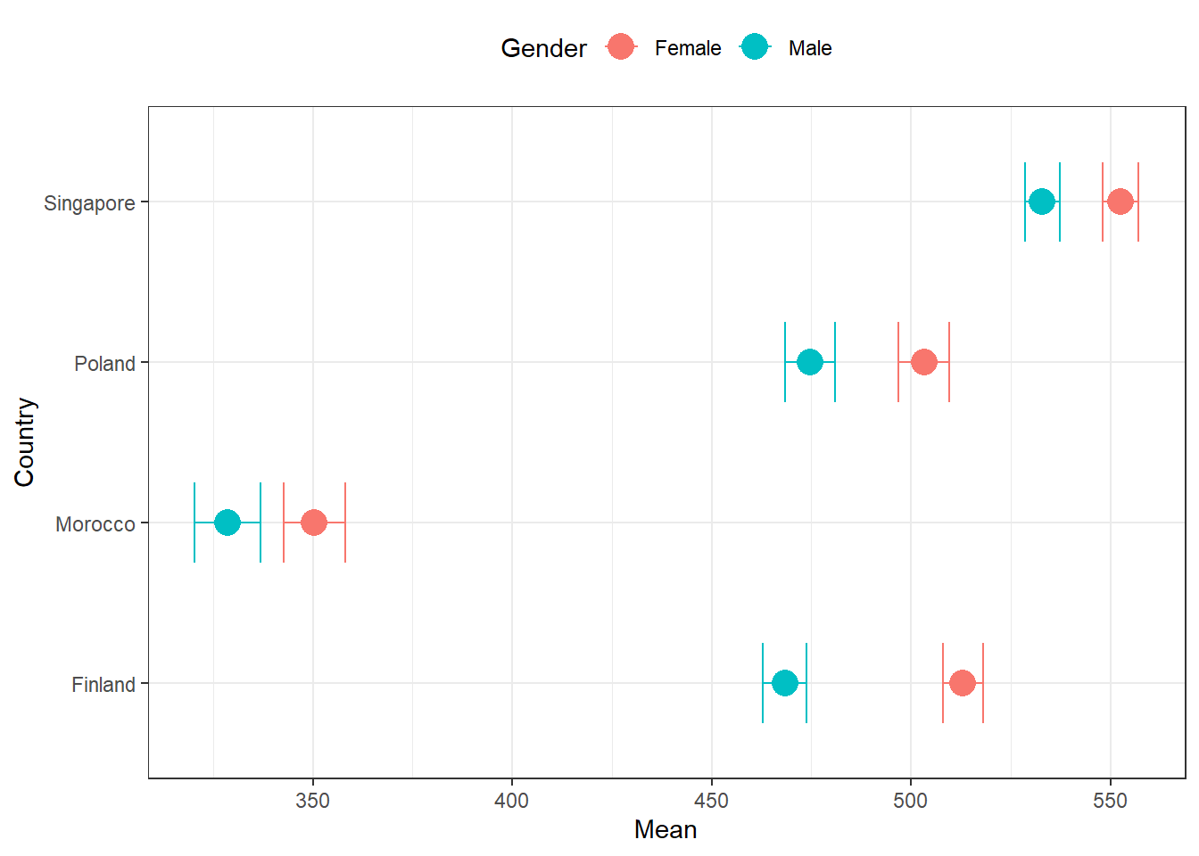
5 Do science skills differ depending on the place of residence?
We will answer this question using linear regression, with science as the outcome variable and the place of residence as the predictor. The “village, hamlet or rural area (fewer than 3 000 people)” will be the reference category.
Recode place of residence variable
dplyr:
Apart from base R, we will also use the dplyr package for data manipulation. The dplyr package uses verb functions connected by pipes (%>%). You can read more about the pipe operator here: / Pipe function documentation
The “Pipes” chapter in “R for Data Science”
The place of residence variable (SC001Q01TA) has very long category names.
Let’s add labels to this factor for more readable outputs.
kable(with(pisa22, table(SC001Q01TA)))| SC001Q01TA | Freq |
|---|---|
| A village, hamlet or rural area (fewer than 3 000 people) | 2198 |
| A small town (3 000 to about 15 000 people) | 3059 |
| A town (15 000 to about 100 000 people) | 7538 |
| A city (100 000 to about 1 000 000 people) | 8223 |
| A large city (1 000 000 to about 10 000 000 people) | 8003 |
| A megacity (with over 10 000 000 people) | 380 |
pisa22[["SC001Q01TA"]] <- factor(pisa22[["SC001Q01TA"]],
  levels = c("A village, hamlet or rural area (fewer than 3 000 people)",
             "A small town (3 000 to about 15 000 people)",
             "A town (15 000 to about 100 000 people)",
             "A city (100 000 to about 1 000 000 people)",
             "A large city (1 000 000 to about 10 000 000 people)",
             "A megacity (with over 10 000 000 people)"),
  labels = c(" Rural <3k",
             " Small town 3k-15k",
             " Town 15k-100k",
             " City 100k-1M",
             " Large city 1M-10M",
             " Megacity >10M")
)
Run linear regression model
Significance of the results
To determine if the predictor is significant, we should look at the t-values in the regression output.
A t-value greater than 1.96 (in absolute value) indicate that the predictor is statistically significant at the 0.05 significance level.
Alternatively, we can calculate p-value from the t-value using the following formula:
p-value = 2 * (1 - pt(abs(t-value), df)) where df is the number of replicate weights - number of parameters to estimate.
# The impact of place of residence on science skills
city_lm <- pisa.reg.pv(
  pvlabel = paste0("PV", 1:10, "SCIE"),
  x = c("SC001Q01TA"),
  data = pisa22
)

# set dfs for p value calculation
# 80 replicate weights - 1 (intercept) - 5 levels of the factor (6-1 (reference))
dfs <- 80 - 1 - (length(levels(pisa22[["SC001Q01TA"]])) - 1)

city_lm_tab <- city_lm[["reg"]]
city_lm_tab[["p-value"]] <- 2 * (1 - pt(abs(city_lm_tab[["t value"]]), dfs))
city_lm_tab[["p-value"]] <- ifelse(city_lm_tab[["p-value"]] < 0.001,
                                  "<0.001",
                                  round(city_lm_tab[["p-value"]], 3)
 )
rownames(city_lm_tab) <- c("Intercept", levels(pisa22[["SC001Q01TA"]])[-1], "R²")

kable(city_lm_tab,
      digits = 2,
      col.names = c("Variable", "Estimate", "Std. Error", "t-value", "p-value"),
      align = c("l", "r", "r", "r", "r")
)| Variable | Estimate | Std. Error | t-value | p-value |
|---|---|---|---|---|
| Intercept | 366.81 | 5.78 | 63.47 | <0.001 |
| Small town 3k-15k | 58.93 | 10.39 | 5.67 | <0.001 |
| Town 15k-100k | 84.18 | 8.27 | 10.19 | <0.001 |
| City 100k-1M | 84.70 | 9.42 | 8.99 | <0.001 |
| Large city 1M-10M | 86.85 | 11.04 | 7.87 | <0.001 |
| Megacity >10M | 15.90 | 19.37 | 0.82 | 0.414 |
| R² | 0.07 | 0.01 | 5.36 | <0.001 |
intsvy allows for the plotting of some basic regression coefficients.
However, to plot a regression with a factor predictor, with several levels we have to use another package, such as ggplot2.
First we need to calculate CIs and add a column with color depending on the direction of the effect.
city_lm_plot <- city_lm_tab %>%
   mutate(
    conf.low = Estimate - 1.96 * `Std. Error`,
    conf.high = Estimate + 1.96 * `Std. Error`,
    color = ifelse(Estimate < 0, "#377EB8", "#E41A1C"),
    city = factor(rownames(city_lm_tab), levels = rev(levels(pisa22[["SC001Q01TA"]])[-1]))
  ) %>%
    filter(city != "Intercept" & city != "R²")

city_lm_plot %>%
  ggplot(aes(Estimate, city)) +
  geom_point(aes(colour = color), size = 3) +
  geom_errorbarh(aes(xmin = conf.low, xmax = conf.high, colour = color), linewidth = 1.5, height = 0.2) +
  geom_vline(xintercept = 0, lty = 2) +
  labs(
    x = "Effect on science results vs rural areas (<3k residents)",
    y = "Place of residence"
      ) +
  scale_colour_manual(values = unique(as.character(city_lm_plot[["color"]]))) +
  theme_minimal(base_size = 10) +
  theme(legend.position = "none")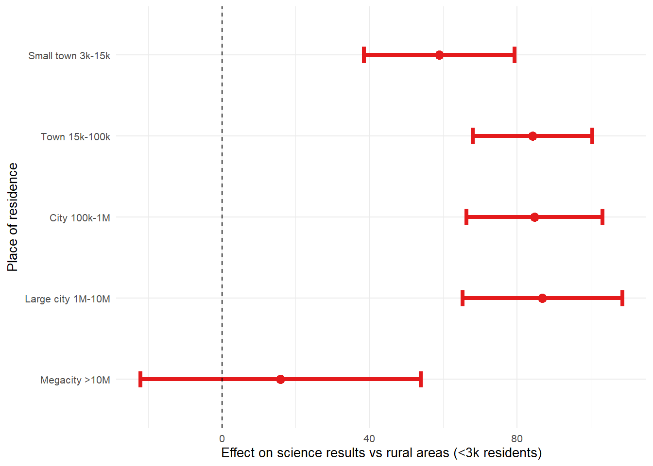
6 SES as a predictor of being absent from school for 3+ months due to problematic behavior
In this section, we will use logistic regression to examine whether socioeconomic status (SES) predicts the likelihood of missing school for 3 or more months due to problematic behavior.
Cross table for country and the variable of interest
First we should look at the cross table for the country and the variable of interest (ST261Q02JA).
cross_tab <- with(pisa22, table(CNT, ST261Q02JA))
kable(cross_tab, digits = 2,
  col.names = c("Country", "Yes, n", "No, n")
)| Country | Yes, n | No, n |
|---|---|---|
| Finland | 34 | 250 |
| Morocco | 116 | 812 |
| Poland | 29 | 264 |
| Singapore | 18 | 272 |
prop_tab <- prop.table(cross_tab, margin = 1) * 100
kable(prop_tab, digits = 2,
  col.names = c("Country", "Yes, %", "No, %")
)| Country | Yes, % | No, % |
|---|---|---|
| Finland | 11.97 | 88.03 |
| Morocco | 12.50 | 87.50 |
| Poland | 9.90 | 90.10 |
| Singapore | 6.21 | 93.79 |
The proportion of students who missed school for 3 or more months due to problematic behavior is relatively low across all countries, but there are noticeable differences.
Singapore has the lowest proportion (6.2%), while in Morocco the proportion is the highest (12.5%).
Nevertheless, we want to examine if SES predicts problematic behavior in these 4 countries.
Running the logistic regression model
# Probability of missing school due to problematic behavior by SES
escs_log <- pisa.log(
  y = "ST261Q02JA",
  x = "ESCS",
  by = "CNT",
  data = pisa22
)

# set dfs for p value calculation
# 80 replicate weights - 1 (intercept) - 1 (predictor)
dfs_log <- 80 - 1 - 1

escs_all_log <- do.call(rbind, list(escs_log[["Finland"]][["reg"]],
                                    escs_log[["Morocco"]][["reg"]],
                                    escs_log[["Poland"]][["reg"]],
                                    escs_log[["Singapore"]][["reg"]]
                                    )
                        )

escs_all_log[["p-value"]] <- 2 * (1 - pt(abs(escs_all_log[["t value"]]), dfs_log))
escs_all_log[["p-value"]] <- ifelse(escs_all_log[["p-value"]] < 0.001,
                                  "<0.001",
                                  round(escs_all_log[["p-value"]], 3)
 )

rownames(escs_all_log) <- paste0(rep(c("Finland", "Morocco", "Poland", "Singapore"), each = 2), c(" Intercept", ""))

kable(escs_all_log,
      digits = 2,
      col.names = c("Variable","Estimate", "Std. Error", "t-value", "Odds Ratio", "lower CI95", "upper CI95", "p-value"),
      row.names = TRUE,
      align = c("l", "r", "r", "r", "r", "r", "r", "r")
) | Variable | Estimate | Std. Error | t-value | Odds Ratio | lower CI95 | upper CI95 | p-value |
|---|---|---|---|---|---|---|---|
| Finland Intercept | 2.11 | 0.26 | 8.11 | 8.28 | 4.97 | 13.80 | <0.001 |
| Finland | -0.49 | 0.21 | -2.32 | 0.61 | 0.40 | 0.93 | 0.023 |
| Morocco Intercept | 1.27 | 0.16 | 7.91 | 3.56 | 2.60 | 4.88 | <0.001 |
| Morocco | -0.45 | 0.08 | -5.47 | 0.64 | 0.54 | 0.75 | <0.001 |
| Poland Intercept | 2.24 | 0.25 | 8.87 | 9.36 | 5.71 | 15.35 | <0.001 |
| Poland | -0.05 | 0.40 | -0.12 | 0.95 | 0.44 | 2.07 | 0.904 |
| Singapore Intercept | 2.98 | 0.28 | 10.49 | 19.72 | 11.29 | 34.42 | <0.001 |
| Singapore | 0.56 | 0.27 | 2.07 | 1.74 | 1.03 | 2.95 | 0.041 |
As with the linear regression plot, we also have to use ggplot2 to prepare the plot for logistic regression.
escs_log_plot <- escs_all_log %>%
   mutate(
    conf.low = `Coef.` - 1.96 * `Std. Error`,
    conf.high = `Coef.` + 1.96 * `Std. Error`,
    color = ifelse(`Coef.` < 0, "#377EB8", "#E41A1C"),
    country = rownames(escs_all_log)
  ) %>%
    filter(!(endsWith(country, "Intercept")))

escs_log_plot %>%
  ggplot(aes(`Coef.`, country)) +
  geom_point(aes(colour = color), size = 3) +
  geom_errorbarh(aes(xmin = conf.low, xmax = conf.high, colour = color), linewidth = 1.5, height = 0.2) +
  geom_vline(xintercept = 0, lty = 2) +
  labs(
    x = "Effect of SES on missing school for >3 months due to problematic behavior",
    y = "Country"
      ) +
  scale_colour_manual(values = unique(as.character(escs_log_plot[["color"]]))) +
  theme_minimal(base_size = 10) +
  theme(legend.position = "none")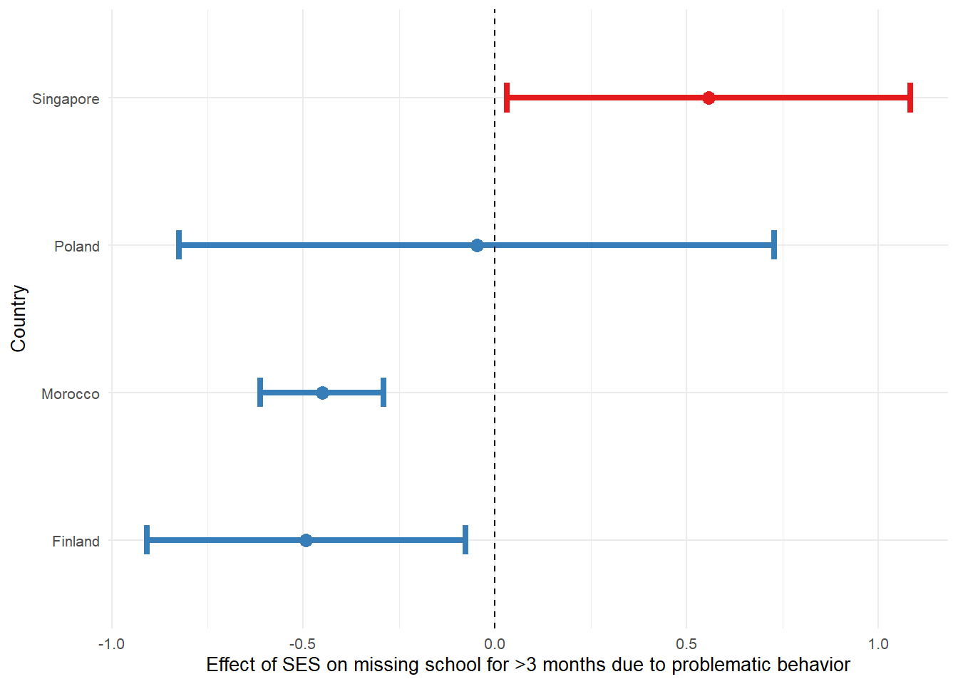
7 Summary
This document demonstrates how to prepare and analyze the PISA 2022 study using the R intsvy package. We covered data loading and merging, and conducting descriptive statistics and regression analyses while accounting for the complex survey design. The results provide insights into differences in reading skills by country and gender. Next, we explore the relationship between the size of the place of residence and science skills. Lastly, we examine the impact of socio-economic status on the probability of missing school due to problematic behavior.