library(haven) # for reading .dta Stata files
library(dplyr) # for data manipulation
library(tidyr) # for data reshaping
library(labelled) # for removing variable labels
library(Rrepest) # for complex survey analysis
library(knitr) # for creating pretty html tables
library(ggplot2) # for data visualization

# Set data path to your data directory
data_path <- "data/SSES/"

# Set the vector with column names containing replication weights
weights_vec <- paste0("rwgt", 1:76)SSES case study analysis with Rrepest
Assessing the effects of gender, site, and age cohort on self-control and empathy and the effect of SES on high empathy. Descriptive statistics, linear and logistic regression analyses are utilized in the tutorial.
1 Introduction
This document demonstrates the preparation and analysis of the SSES 2019 (Survey on Social and Emotional Skills 2019) dataset using R. SSES 2019 was the first edition of an international educational study aimed at assessing the social and emotional skills of 10- and 15-year-old students.
The analysis presented here focuses on gender, site, and age cohort differences in self-control and the relationship between socioeconomic status (SES) and high empathy.
We will use the student dataset, focusing on a subset of sites: Bogota, Helsinki, and Moscow.
2 Setup
First, let’s load the required packages and set up our environment:
3 Data download and loading
Data download
The data can be downloaded from the SSES 2019 public data repository.
You need to download INT_01_ST_(2021.04.14)_Public.dta (a Stata data format) file from the SSES 2019 public data repository and place it in the chosen directory.
The .sav file (an SPSS data format) is also there, but the students dataset in .sav is missing one replicating weight (rwgt9), thus it is not useful.
The variables we will focus on are:
Gender_Std- student’s gender (1 = female, 2 = male)CohortID- cohort of students (1 = 10 years old, 2 = 15 years old)SiteID- site identification numberSES- socioeconomic background scoreSEL_WLE_ADJ- self-control scoreEMP_WLE_ADJ- empathy score
We will read the raw data files and select only the variables we need for the analysis:
# Read raw data
student_data <- read_dta(paste0(data_path, "INT_01_ST_(2021.04.14)_Public.dta"))

# Define variables to keep
student_vars <- c("Username_Std", "Username_TC", "SiteID", "Gender_Std", "CohortID",
                  "SEL_WLE_ADJ", "EMP_WLE_ADJ", "SES", weights_vec, "WT2019")
4 Data manipulation using dplyr
The dplyr package uses verb functions connected by pipes (%>%).
You can read more about pipe operator here:
# Choose only Males and Females
sses_data <- student_data %>%
  filter(Gender_Std %in% c(1,2))

# Choose columns (variables) needed for analysis
sses_data <- sses_data %>%
  select(all_of(student_vars))

# Filter only 3 sites and create transformations
sses_data <- sses_data %>%
  filter(SiteID %in% c("01", "03", "07")) %>% # Choose Bogota, Helsinki and Moscow
  mutate(
    # Create a variable with site names instead of numbers
    SiteName = case_when(
      SiteID == "01" ~ "Bogota",
      SiteID == "03" ~ "Helsinki",
      SiteID == "07" ~ "Moscow"
    ),
    # Change Gender to binary variable
    Gender_Std = if_else(Gender_Std == 1, 0, 1),
    Gender = if_else(Gender_Std == 0, "Female", "Male"),
    CohortID = if_else(CohortID == 1, 0, 1),
    Cohort_name = if_else(CohortID == 0, "10 y.o.", "15 y.o.")
  )

# Remove labels
sses_data <- remove_labels(sses_data)
We have the dataset ready for analysis. Let’s proceed.
5 Differences in self-control between sites and genders
In this section, we will compare means and standard deviations of self-control score (SEL_WLE_ADJ) by Site and Gender.
However, first is a brief description of the Rrepest package and its main function.
Description of the commonly used Rrepest() arguments:
svyargument specifies the survey design
byargument allows grouping by multiple variables
estargument specifies the statistics to calculate (e.g., mean, standard deviation);
targetspecifies the variable for which statistics are calculated (e.g.,SEL_WLE_ADJfor self-control)
Note
More about the Rrepest package can be found in our tutorial.
Mean and standard deviation of self-control by site and gender
# run descriptive statistics
desc_results <- Rrepest(sses_data,
        svy = "SSES",
        by = c("SiteName", "Gender"),
        est = est(c("mean", "std"), target = "SEL_WLE_ADJ")
)

# plot table
kable(desc_results,
  digits = 2,
  col.names = c("Site", "Gender", "Mean", "Mean SE", "SD", "SD SE"),
  align = c("l", "l", "r", "r", "r", "r")
)| Site | Gender | Mean | Mean SE | SD | SD SE |
|---|---|---|---|---|---|
| Bogota | Female | 578.07 | 1.50 | 90.11 | 2.25 |
| Bogota | Male | 559.93 | 1.88 | 85.02 | 1.85 |
| Helsinki | Female | 581.43 | 2.00 | 94.14 | 2.40 |
| Helsinki | Male | 578.30 | 2.09 | 92.61 | 1.74 |
| Moscow | Female | 564.53 | 1.68 | 89.00 | 1.57 |
| Moscow | Male | 577.64 | 1.66 | 93.39 | 1.67 |
We can also present the results on a bar plot:
# plot barplot
desc_results %>%
  ggplot(aes(x = SiteName, y = b.mean.sel_wle_adj, fill = Gender)) +
  geom_bar(stat="identity", color="black", position=position_dodge()) +
  scale_fill_brewer(palette="Set1") +
  xlab("Site") +
  ylab("Mean Self-Control Score") +
  theme_minimal(base_size = 14)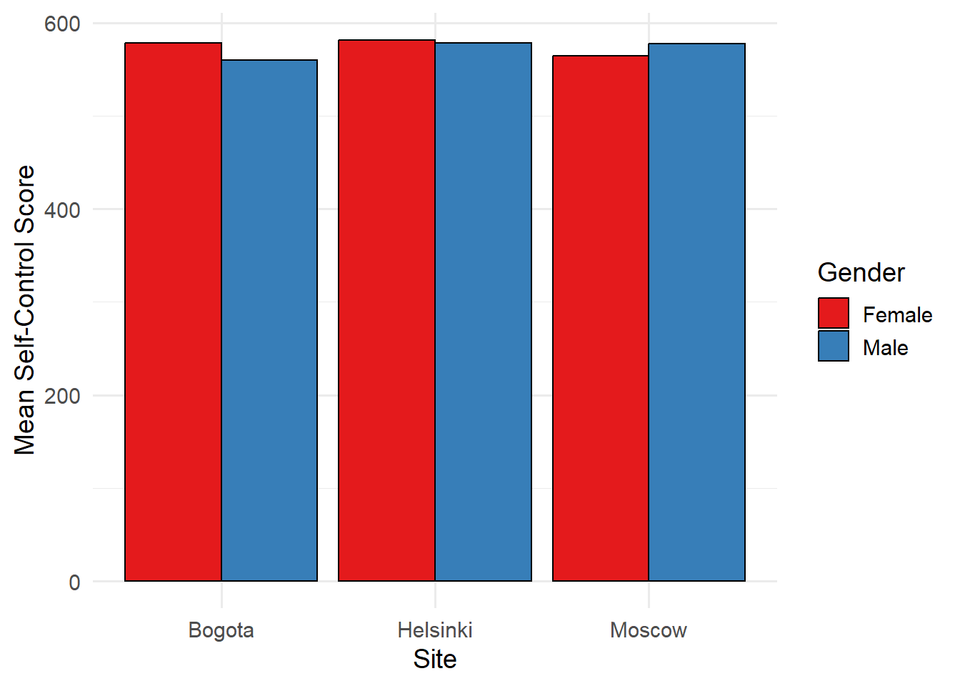
6 Does self-control differ by age cohort?
We will answer this question using linear regression, with self-control as the outcome variable and age cohort (10 vs 15 years old) as the predictor.
Using Rrepest we will:
- Perform weighted linear regression
- Extract and format regression coefficients, standard errors, and R-square statistics
- Calculate t-statistics manually for hypothesis testing
Significance Testing
To determine if the predictor is significant, we should look at the t-values in the regression output.
A t-value greater than 1.96 (in absolute value) indicates that the predictor is statistically significant at the 0.05 significance level.
Alternatively, we can calculate p-value from the t-value using the following formula:
p-value = 2 * (1 - pt(abs(t-value), df)) where df is the number of replicate weights - number of parameters to estimate.
To calculate the t-statistic for the regression table we have to set the number of degrees of freedom.
Degrees of freedom are equal to the number of replication weights minus the number of parameters estimated.
In both regression analyses we have two parameters: intercept and 1 regressor (CohortID - age cohort).
n_dfs <- 76 - 2Run linear regression model
lm_results <- Rrepest(data = sses_data,
        svy = "SSES",
        by = "SiteName",
        est = est("lm",
                  target = "SEL_WLE_ADJ",
                  regressor = 'CohortID'))
Next, we will create a formatted regression table using dplyr and tidyr:
# reshape the results table
lm_reshaped <- lm_results %>%
  pivot_longer(
    cols = -SiteName,
    names_to = c("stat_type", "parameter"),
    names_pattern = "^(b\\.|se\\.)reg_sel_wle_adj\\.(.+)$",
    values_to = "value"
  ) %>%
  mutate(
    stat_type = case_when(
      stat_type == "b." ~ "Estimate",
      stat_type == "se." ~ "SE"
    ),
    parameter = case_when(
      parameter == "intercept" ~ "Intercept",
      parameter == "cohortid" ~ "Cohort Age",
      parameter == "rsqr" ~ "R²"
    )
  ) %>%
  pivot_wider(
    names_from = stat_type,
    values_from = value
  ) %>%
  select(SiteName, parameter, Estimate, SE) %>%
  mutate(
    t_value = Estimate / SE,
    conf.low = Estimate - 1.96 * SE,
    conf.high = Estimate + 1.96 * SE,
    p_value = 2 * pt(abs(t_value), n_dfs, lower.tail = FALSE),
    p_value = ifelse(p_value < 0.001, "<0.001", format(round(p_value, 3), digits = 3, nsmall = 3))
    )

# reshape for plot
lm_for_plot <- lm_reshaped %>%
  filter(parameter == "Cohort Age") %>%
  select(SiteName, Estimate, SE, conf.low, conf.high) %>%
  mutate(
    color = ifelse(Estimate < 0, "#377EB8", "#E41A1C")
  )
# reshape for html table
lm_reshaped <- lm_reshaped %>%
  mutate(
    SiteName = ifelse(duplicated(SiteName), "", SiteName),
    conf.low = ifelse(conf.low > -0.01 & conf.low < 0, "<0", format(round(conf.low, 2), digits = 2, nsmall = 2)),
    conf.high = ifelse(conf.high < 0.01, "<0.01", format(round(conf.high, 2), digits = 2, nsmall = 2))
  )

# plot table
kable(lm_reshaped,
  digits = 2,
  col.names = c("Site", "Parameter", "Estimate", "Std. Error", "t-value", "lower CI", "upper CI", "p-value"),
    align = c("l", "l", "r", "r", "r", "r", "r", "r")

)| Site | Parameter | Estimate | Std. Error | t-value | lower CI | upper CI | p-value |
|---|---|---|---|---|---|---|---|
| Bogota | Intercept | 573.56 | 1.89 | 304.13 | 569.86 | 577.25 | <0.001 |
| Cohort Age | -8.87 | 2.86 | -3.10 | -14.47 | <0.01 | 0.003 | |
| R² | 0.00 | 0.00 | 1.58 | <0 | <0.01 | 0.119 | |
| Helsinki | Intercept | 591.82 | 2.84 | 208.39 | 586.26 | 597.39 | <0.001 |
| Cohort Age | -25.98 | 3.38 | -7.69 | -32.60 | <0.01 | <0.001 | |
| R² | 0.02 | 0.00 | 4.05 | 0.01 | 0.03 | <0.001 | |
| Moscow | Intercept | 571.95 | 2.07 | 275.76 | 567.89 | 576.02 | <0.001 |
| Cohort Age | -1.55 | 2.78 | -0.56 | -7.00 | 3.90 | 0.579 | |
| R² | 0.00 | 0.00 | 0.27 | <0 | <0.01 | 0.786 |
Below is a plot showing the estimates and 95% confidence intervals for the effect of age cohort on self-control by site.
All the estimates are negative, thus the color blue was used.
You can see that for Bogota and Helsinki the confidence intervals do not cross zero, thus the effect is significant.
For Moscow the confidence interval crosses zero, thus the effect is not significant.
# make linear regression estimates plot
lm_for_plot %>%
  ggplot(aes(Estimate, SiteName)) +
  geom_point(aes(colour = color), size = 3) +
  geom_errorbarh(aes(xmin = conf.low, xmax = conf.high, colour = color), linewidth = 1.5, height = 0.2) +
  geom_vline(xintercept = 0, lty = 2) +
  labs(
    x = "Estimate of the effect of Age cohort on self-control (15 y.o. vs 10 y.o.)",
    y = "Site"
      ) +
  scale_colour_manual(values = unique(as.character(lm_for_plot[["color"]]))) +
  theme_minimal(base_size = 9) +
  theme(legend.position = "none")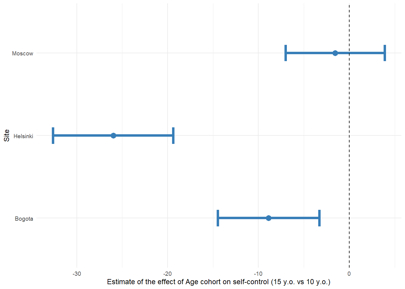
7 SES as predictor of high empathy
In this section, we will use logistic regression to examine whether socioeconomic status (SES) predicts high empathy (EMP_WLE_ADJ). We will define high empathy as scoring above the 90th percentile of the empathy score distribution.
Create the binary variable for high empathy and run the logistic regression
# Calculate the 90th percentile empathy score
emp_90 <- quantile(sses_data$EMP_WLE_ADJ, 0.9, na.rm = TRUE)

# Create binary variable for high empathy
sses_data[["emp_90_bin"]] <- ifelse(sses_data[["EMP_WLE_ADJ"]] < emp_90, 0, 1)

# Run logistic regression
log_results <- Rrepest(
  data = sses_data,
  svy = "SSES",
  est = est("log",
            target = 'emp_90_bin',
            regressor = "SES"),
  by = "SiteName"
)
As before, we will create a formatted regression table using dplyr:
# reshape the results table
log_reshaped <- log_results %>%
  pivot_longer(
    cols = -SiteName,
    names_to = c("stat_type", "parameter"),
    names_pattern = "^(b\\.|se\\.)log_emp_90_bin\\.(.+)$",
    values_to = "value"
  ) %>%
  mutate(
    stat_type = case_when(
      stat_type == "b." ~ "Estimate",
      stat_type == "se." ~ "SE"
    ),
    parameter = case_when(
      parameter == "intercept" ~ "Intercept",
      parameter == "ses" ~ "SES"
    )
  ) %>%
  pivot_wider(
    names_from = stat_type,
    values_from = value
  ) %>%
  select(SiteName, parameter, Estimate, SE) %>%
  mutate(
    t_value = Estimate / SE,
    conf.low = Estimate - 1.96 * SE,
    conf.high = Estimate + 1.96 * SE,
    p_value = 2 * pt(abs(t_value), n_dfs, lower.tail = FALSE),
    p_value = ifelse(p_value < 0.001, "<0.001", round(p_value, 3))
  )

# reshape for plot
log_for_plot <- log_reshaped %>%
  filter(parameter == "SES") %>%
  select(SiteName, Estimate, SE, conf.low, conf.high) %>%
  mutate(
    color = ifelse(Estimate < 0, "#377EB8", "#E41A1C")
  )

# reshape for html table
log_reshaped <- log_reshaped %>%
  mutate(
    SiteName = ifelse(duplicated(SiteName), "", SiteName)
  )

# plot html table
kable(log_reshaped,
  digits = 2,
  col.names = c("Site", "Parameter", "Estimate", "Std. Error", "t-value", "lower CI", "upper CI", "p-value"),
  align = c("l", "l", "r", "r", "r", "r", "r", "r")
)| Site | Parameter | Estimate | Std. Error | t-value | lower CI | upper CI | p-value |
|---|---|---|---|---|---|---|---|
| Bogota | Intercept | -2.39 | 0.09 | -26.29 | -2.57 | -2.21 | <0.001 |
| SES | 0.26 | 0.06 | 4.03 | 0.13 | 0.39 | <0.001 | |
| Helsinki | Intercept | -2.46 | 0.04 | -56.73 | -2.54 | -2.37 | <0.001 |
| SES | 0.39 | 0.05 | 8.52 | 0.30 | 0.48 | <0.001 | |
| Moscow | Intercept | -2.47 | 0.08 | -30.98 | -2.63 | -2.32 | <0.001 |
| SES | 0.52 | 0.08 | 6.88 | 0.37 | 0.66 | <0.001 |
As before, we will create a plot showing the odds ratios and 95% confidence intervals for the effect of SES on high empathy by site.
None of the estimates cross zero, thus the effect is significant in all sites.
All of the estimates are positive, thus the color red was used.
# make log regression estimates plot
log_for_plot %>%
  ggplot(aes(Estimate, SiteName)) +
  geom_point(aes(colour = color), size = 3) +
  geom_errorbarh(aes(xmin = conf.low, xmax = conf.high, colour = color), linewidth = 1.5, height = 0.2) +
  geom_vline(xintercept = 0, lty = 2) +
  labs(
    x = "Estimate of the effect of SES on the probability of empathy score\nover 90 percentile",
    y = "Site"
      ) +
  scale_colour_manual(values = unique(as.character(log_for_plot[["color"]]))) +
  theme_minimal(base_size = 9) +
  theme(legend.position = "none")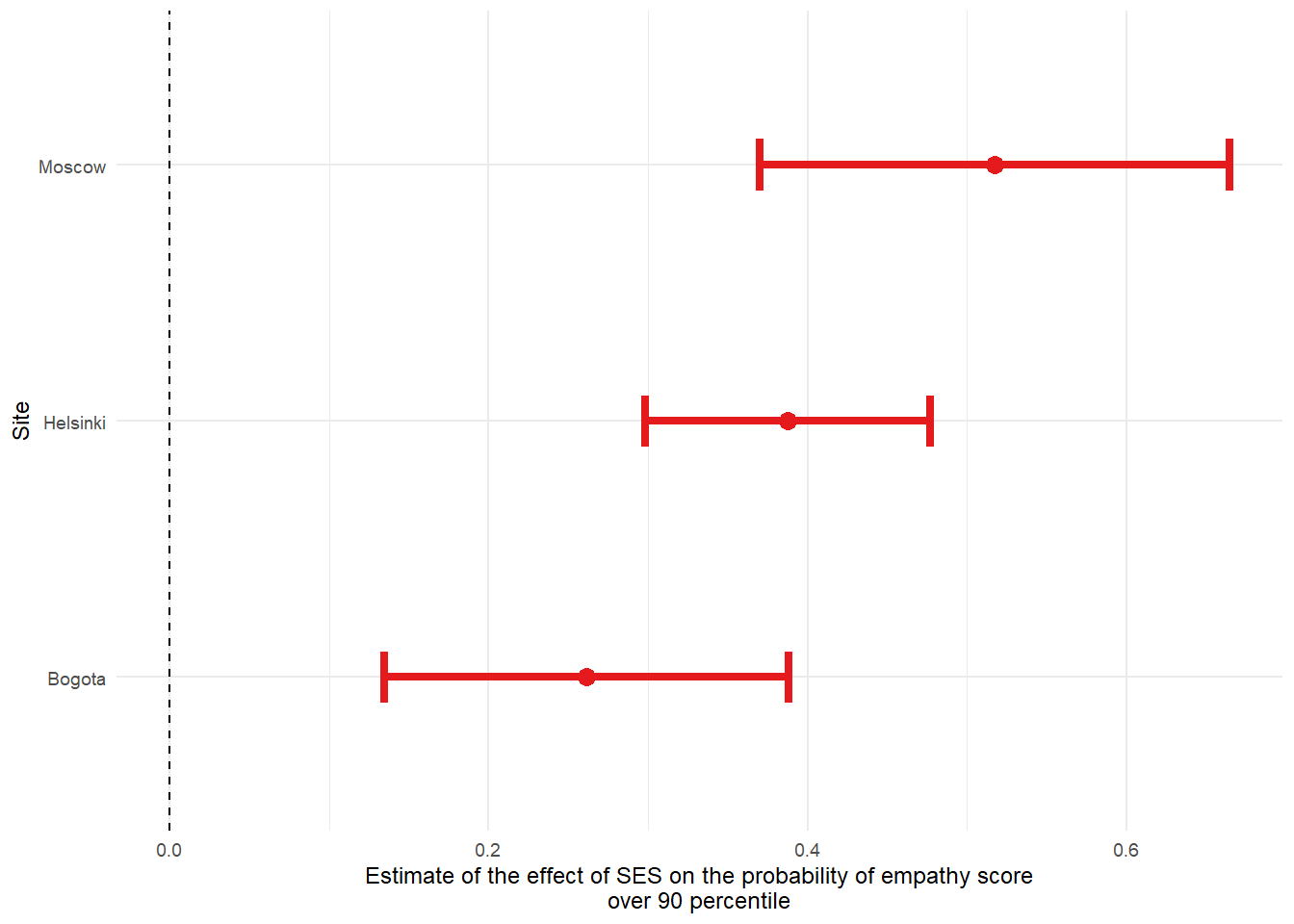
8 Summary
This document demonstrates how to prepare and analyze SSES 2019 data using R and the Rrepest package. We cover data loading, manipulation with dplyr, and conducting descriptive statistics and regression analyses while accounting for the complex survey design. The results provide insights into differences in self-control by site, gender, and age cohort, as well as the relationship between socioeconomic status and high empathy.